One way Anova manually in r

On This Page

Model
Required ANOVA Table
Example
ANOVA Summary Table
Conclusion
R code

One-Way ANOVA (Analysis of Variance) is a statistical test used to determine if there are any statistically significant differences between the means of three or more independent (unrelated) groups.

Let $Y_{ij}$ be the $j$ th observation of $i$ th group . We can write the model as

Model

\[Y_{ij} = \mu + \tau_i + \epsilon_{ij}\]

$Y_{ij}$: The observation from group $i$ and individual $j$
$\mu$: The overall mean
$\tau_i$: The effect of the $i$-th group
$\epsilon_{ij}$: The random error term

Now using LSE of $\mu , \alpha_i,\epsilon_{ij} $ The reduced model assumes that there are no differences between group means:

\[Y_{ij} = \mu + \epsilon_{ij}\]

Required ANOVA Table

The ANOVA summary table partitions the total variation into components due to the model (between groups) and error (within groups).

Source	Sum of Squares (SS)	Degrees of Freedom (df)	Mean Square (MS)	F-statistic
Between Groups	$SSB$	$k-1$	$MSB = \frac{SSB}{k-1}$	$F = \frac{MSB}{MSW}$
Within Groups	$SSW$	$N-k$	$MSW = \frac{SSW}{N-k}$
Total	$SST$	$N-1$

$SSB$: Between-group sum of squares
$SSW$: Within-group sum of squares
$SST$: Total sum of squares ($SST = SSB + SSW$)
$k$: Number of groups
$N$: Total number of observations

Example

Consider the following data:

Group 1: $1, 2, 5$
Group 2: $2, 4, 2$
Group 3: $2, 3, 4$

Calculate Group Means and Overall Mean

Group 1 mean: $\mu_1 = \frac{1 + 2 + 5}{3} = 2.67$
Group 2 mean: $\mu_2 = \frac{2 + 4 + 2}{3} = 2.67$
Group 3 mean: $\mu_3 = \frac{2 + 3 + 4}{3} = 3.00$
Overall mean: $\mu = \frac{1 + 2 + 5 + 2 + 4 + 2 + 2 + 3 + 4}{9} = 2.78$

Compute the Sum of Squares

\[SSB = \sum_{i=1}^{k} n_i (\mu_i - \mu)^2\]

where $n_i$ is the number of observations in group $i$.

\[SSB = 3(2.67 - 2.78)^2 + 3(2.67 - 2.78)^2 + 3(3.00 - 2.78)^2\] \[SSB = 3 \times (-0.11)^2 + 3 \times (-0.11)^2 + 3 \times 0.22^2\] \[SSB = 0.3636\]

Within-group sum of squares

\[SSW = \sum_{i=1}^{k} \sum_{j=1}^{n_i} (Y_{ij} - \mu_i)^2\]

For Group 1:

\[SSW_1 = (1 - 2.67)^2 + (2 - 2.67)^2 + (5 - 2.67)^2 = 2.7889 + 0.4489 + 5.4489 = 8.6867\]

For Group 2:

\[SSW_2 = (2 - 2.67)^2 + (4 - 2.67)^2 + (2 - 2.67)^2 = 0.4489 + 1.7689 + 0.4489 = 2.6667\]

For Group 3:

\[SSW_3 = (2 - 3.00)^2 + (3 - 3.00)^2 + (4 - 3.00)^2 = 1 + 0 + 1 = 2\] \[SSW = SSW_1 + SSW_2 + SSW_3 = 8.6867 + 2.6667 + 2 = 13.3534\]

Now calculate Mean squares and F statistics in ANOVA table

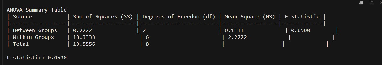
ANOVA Summary Table

Source	Sum of Squares (SS)	Degrees of Freedom (df)	Mean Square (MS)	F-statistic
Between Groups	0.3636	2	SSB/2= 0.1818	0.0817
Within Groups	13.3534	6	SSW/6 2.2256
Total	13.717	8

Conclusion

Compare the F-statistic to the critical value from the F-distribution table at a chosen significance level (e.g., $\alpha = 0.05$). For $df_1 = 2$ and $df_2 = 6$, the critical value is approximately 5.14. Since 0.0817 < 5.14, we fail to reject the null hypothesis and conclude that there are no significant differences between the group means.

Ref:

R code

data <- data.frame(
  group1 = c(1, 2, 5),
  group2 = c(2, 4, 2),
  group3 = c(2, 3, 4)
)
# Calculate group means
group_means <- c(mean(data$group1), mean(data$group2), mean(data$group3))
# Calculate overall mean
overall_mean <- mean(unlist(data))
# Number of groups and total number of observations
k <- ncol(data)
N <- length(unlist(data))
# Calculate Sum of Squares Between (SSB)
ssb <- 0
for (i in 1:k) {
  ssb <- ssb + length(data[, i]) * (group_means[i] - overall_mean)^2
}
# Calculate Sum of Squares Within (SSW)
ssw <- 0
for (i in 1:k) {
  ssw <- ssw + sum((data[, i] - group_means[i])^2)
}
# Calculate Total Sum of Squares (SST)
sst <- ssw + ssb
# Degrees of Freedom
df_between <- k - 1
df_within <- N - k
df_total <- df_between + df_within
# Mean Squares
msb <- ssb / df_between
msw <- ssw / df_within
# F-statistic
f_statistic <- msb / msw

R output