One way ANOVA in R

Prepare Data

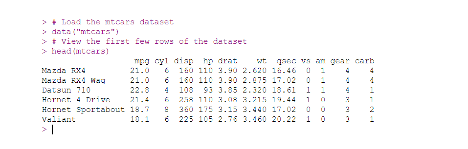
For this tutorial, we will use a built-in dataset mtcars in R. This dataset contains data on various car models, including variables like miles per gallon (mpg), number of cylinders (cyl), horsepower (hp), and more.

# Load the mtcars dataset
data("mtcars")
# View the first few rows of the dataset
head(mtcars)

Check Assumptions

ANOVA has several assumptions:

1. Independence: The samples must be independent.
2. Normality: The dependent variable should be approximately normally distributed within each group.
3. Homogeneity of variances: The variances among the groups should be approximately equal.

1. Check for Normality

We can use the Shapiro-Wilk test to check for normality.

# Shapiro-Wilk test for normality
shapiro.test(mtcars$mpg)

shapiro.test(mtcars$mpg)
	Shapiro-Wilk normality test
data:  mtcars$mpg
W = 0.94756, p-value = 0.1229

Interpretation

Null Hypothesis (H0): The data is normally distributed. Alternative Hypothesis (H1): The data is not normally distributed.

p-value = 0.1229 Since the p-value is greater than the common significance level of 0.05, we fail to reject the null hypothesis. We can assume the mpg data is approximately normally distributed.

2. Check for Homogeneity of Variances

The Bartlett test can be used to check for homogeneity of variances.

# Bartlett test for homogeneity of variances
bartlett.test(mpg ~ cyl, data = mtcars)

	Bartlett test of homogeneity of variances
data:  mpg by cyl
Bartlett's K-squared = 8.3934, df = 2, p-value = 0.01505

Interpretation Null Hypothesis (H0): The variances of the different groups are equal. Alternative Hypothesis (H1): At least one group has a variance different from the others.

p-value = 0.01505 Since the p-value is less than the common significance level of 0.05, we reject the null hypothesis.In this case, the variances of mpg among different cylinder groups (cyl) are not equal.

As normality assumption holds, the homogeneity of variances assumption does not. However, ANOVA can still be performed with caution, and alternative approaches or additional steps can be considered to account for the violation of variance homogeneity.

Perform ANOVA

Now, we perform the ANOVA test. We will compare the miles per gallon (mpg) across different numbers of cylinders (cyl).

# Perform ANOVA
anova_result <- aov(mpg ~ cyl, data = mtcars)
# Summary of ANOVA
summary(anova_result)

            Df Sum Sq Mean Sq F value   Pr(>F)    
cyl          1  817.7   817.7   79.56 6.11e-10 ***
Residuals   30  308.3    10.3                     
---
Signif. codes:  0 ‘***’ 0.001 ‘**’ 0.01 ‘*’ 0.05 ‘.’ 0.1 ‘ ’ 1

Interpretation of Results

The summary of the ANOVA test will provide the F-statistic and p-value. If the p-value is less than the significance level (usually 0.05), we reject the null hypothesis and conclude that there is a significant difference between the group means.

Null Hypothesis ($H_0$) The null hypothesis states that there are no differences in the group means. In other words, any observed differences in sample means are due to random variation.

Where:

• $\mu_i$ represents the mean of the $i$-th group.
• $k$ is the number of groups.

Alternative Hypothesis ($H_1$) The alternative hypothesis states that at least one group mean is different from the others. This does not specify which group means are different or how many are different, just that not all the group means are equal.

The ANOVA test show a significant effect of the number of cylinders on miles per gallon, with a very small p-value (6.11e-10). This means we reject the null hypothesis and conclude that there is a statistically significant difference in miles per gallon between different numbers of cylinders in the mtcars dataset.